当前位置：搜档网 › dnn and spato_temporal dynamics

dnn and spato_temporal dynamics

Deep Neural Networks predict Hierarchical Spatio-temporal Cortical Dynamics

of Human Visual Object Recognition

Radoslaw M.Cichy ??Aditya Khosla ?Dimitrios Pantazis ?Antonio Torralba ?

Aude Oliva ?

?Massachusetts Institute of Technology ?Free University Berlin

{rmcichy,khosla,pantazis,torralba,oliva }@https://www.sodocs.net/doc/fe4177967.html,

Abstract

The complex multi-stage architecture of cortical visual

pathways provides the neural basis for ef?cient visual ob-ject recognition in humans.However,the stage-wise com-putations therein remain poorly understood.Here,we compared temporal (magnetoencephalography)and spatial (functional MRI)visual brain representations with repre-sentations in an arti?cial deep neural network (DNN)tuned to the statistics of real-world visual recognition.We showed that the DNN captured the stages of human visual process-ing in both time and space from early visual areas towards the dorsal and ventral streams.Further investigation of crucial DNN parameters revealed that while model archi-tecture was important,training on real-world categoriza-tion was necessary to enforce spatio-temporal hierarchical relationships with the brain.Together our results provide an algorithmically informed view on the spatio-temporal dynamics of visual object recognition in the human visual brain.

1.Introduction

Visual object recognition in humans is mediated by com-plex multi-stage processing of visual information emerg-ing rapidly in a distributed network of cortical regions [43,15,5,31,23,26,14].Understanding visual object recog-nition in cortex thus requires a predictive and quantitative model that captures the complexity of the underlying spatio-temporal dynamics [35,36,34].

A major impediment in creating such a model is the highly nonlinear and sparse nature of neural tuning prop-erties in mid-and high-level visual areas [11,44,47]that is dif?cult to capture experimentally,and thus unknown.Pre-vious approaches to modeling object recognition in cortex relied on extrapolation of principles from well understood lower visual areas such as V1[35,36]and strong manual intervention,achieving only modest task performance com-pared to humans.

Here we take an alternative route,constructing and com-paring against brain signals a visual computational model based on deep neural networks (DNNs)[30,32],i.e.,com-puter vision models in which model neuron tuning prop-erties are set by supervised learning without manual inter-vention [30,37].DNNs are the best performing models on computer vision object recognition benchmarks and yield human performance levels on object categorization [38,19].We used a tripartite strategy to reveal the spatio-temporal processing cascade underlying human visual object recog-nition by DNN model comparisons.

First,as object recognition is a process rapidly unfold-ing over time [5,9,41],we compared DNN visual rep-resentations to millisecond resolved magnetoencephalogra-phy (MEG)brain data.Our results delineate,to our knowl-edge for the ?rst time,an ordered relationship between the stages of processing in computer vision model and the time course with which object representations emerge in the hu-man brain.

Second,as object recognition recruits a multitude of dis-tributed brain regions,a full account of object recognition needs to go beyond the analysis of a few pre-de?ned brain regions [1,6,18,21,48],determining the relationship be-tween DNNs and the whole https://www.sodocs.net/doc/fe4177967.html,ing a spatially unbi-ased approach,we revealed a hierarchical relationship be-tween DNNs and the processing cascade of both the ventral and dorsal visual pathway.

Third,interpretation of a DNN-brain comparison de-pends on the factors shaping the DNN fundamentally:the pre-speci?ed model architecture,the training procedure,and the learned task (e.g.object categorization).By com-paring different DNN models to brain data,we demon-strated the in?uence of each of these factors on the emer-gence of similarity relations between DNNs and brains in both space and time.

Together,our results provide an algorithmically in-formed perspective of the spatio-temporal dynamics under-lying visual object recognition in the human brain.1

a r X i v :1601.02970v 1 [c s .C V ] 12 J a n 2016

2.Results

2.1.Construction of a DNN performing at human

level in object categorization

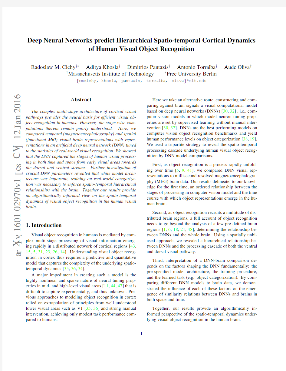
To be a plausible model of object recognition in cor-tex,a computational model must provide high performance on visual object https://www.sodocs.net/doc/fe4177967.html,test generations of com-puter vision models,termed deep neural networks(DNNs), have achieved extraordinary performance,thus raising the question whether their algorithmic representations bear re-semblance of the neural computations underlying human vi-sion.To investigate we created an8-layer DNN architecture (Fig.1(a))that corresponds to the best-performing model in object classi?cation in the ImageNet Large Scale Visual Recognition Challenge2012[29].Each DNN layer per-forms simple operations that are implementable in biologi-cal circuits,such as convolution,pooling and normalization. We trained the DNN to perform object categorization on ev-eryday object categories(683categories,with1300images in each category)using back propagation,i.e.,the network learned neuronal tuning functions by itself.We termed this neural network object deep neural network(object DNN). The object DNN performed equally well on object catego-rization as previous implementations(Suppl.Table1).We investigated the coding of visual information in the object DNN by determining the receptive?eld(RF)selectivity of the model neurons using a neuroscience-inspired reduction method[49].

We found that neurons in early layers had Gabor?lter or color patch-like sensitivity,while those of deeper layers had larger RFs and sensitivity to complex forms(Fig.1(b)). Thus the object DNN learned representations in a hierar-chy of increasing complexity,akin to representations in the primate visual brain hierarchy[23,14].Figure1(c)ex-empli?es the connectivity and receptive?eld selectivity of the most strongly connected neurons starting from a sample neuron in layer1.An online tool offering visualization of RF selectivity of all neurons in layers1through5is avail-able at https://www.sodocs.net/doc/fe4177967.html,.

2.2.Representational similarity analysis was used

as the integrative framework for DNN-brain

comparison

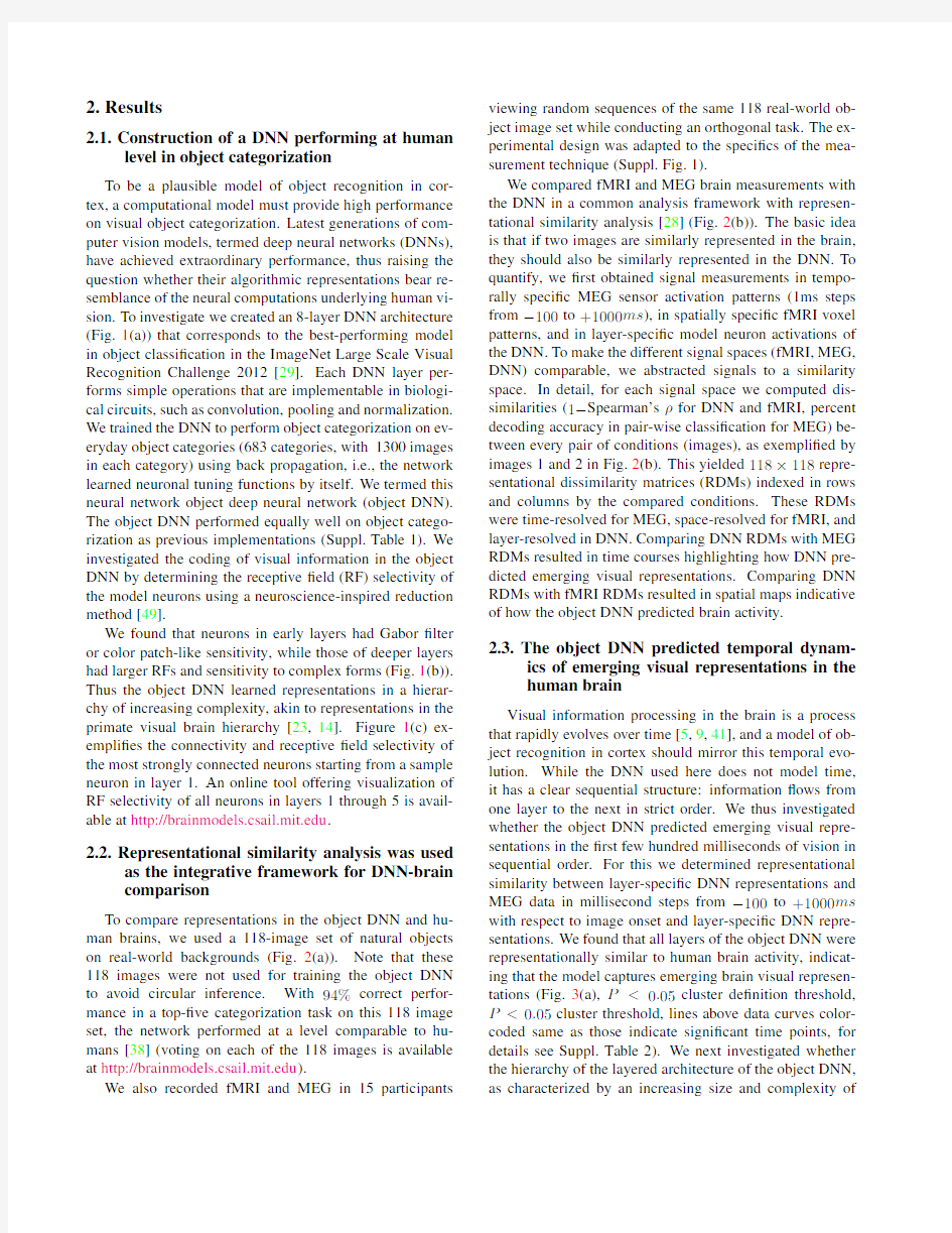
To compare representations in the object DNN and hu-man brains,we used a118-image set of natural objects on real-world backgrounds(Fig.2(a)).Note that these 118images were not used for training the object DNN to avoid circular inference.With94%correct perfor-mance in a top-?ve categorization task on this118image set,the network performed at a level comparable to hu-mans[38](voting on each of the118images is available at https://www.sodocs.net/doc/fe4177967.html,).

We also recorded fMRI and MEG in15participants viewing random sequences of the same118real-world ob-ject image set while conducting an orthogonal task.The ex-perimental design was adapted to the speci?cs of the mea-surement technique(Suppl.Fig.1).

We compared fMRI and MEG brain measurements with the DNN in a common analysis framework with represen-tational similarity analysis[28](Fig.2(b)).The basic idea is that if two images are similarly represented in the brain, they should also be similarly represented in the DNN.To quantify,we?rst obtained signal measurements in tempo-rally speci?c MEG sensor activation patterns(1ms steps from?100to+1000ms),in spatially speci?c fMRI voxel patterns,and in layer-speci?c model neuron activations of the DNN.To make the different signal spaces(fMRI,MEG, DNN)comparable,we abstracted signals to a similarity space.In detail,for each signal space we computed dis-similarities(1?Spearman’sρfor DNN and fMRI,percent decoding accuracy in pair-wise classi?cation for MEG)be-tween every pair of conditions(images),as exempli?ed by images1and2in Fig.2(b).This yielded118×118repre-sentational dissimilarity matrices(RDMs)indexed in rows and columns by the compared conditions.These RDMs were time-resolved for MEG,space-resolved for fMRI,and layer-resolved in https://www.sodocs.net/doc/fe4177967.html,paring DNN RDMs with MEG RDMs resulted in time courses highlighting how DNN pre-dicted emerging visual https://www.sodocs.net/doc/fe4177967.html,paring DNN RDMs with fMRI RDMs resulted in spatial maps indicative of how the object DNN predicted brain activity.

2.3.The object DNN predicted temporal dynam-

ics of emerging visual representations in the

human brain

Visual information processing in the brain is a process that rapidly evolves over time[5,9,41],and a model of ob-ject recognition in cortex should mirror this temporal evo-lution.While the DNN used here does not model time, it has a clear sequential structure:information?ows from one layer to the next in strict order.We thus investigated whether the object DNN predicted emerging visual repre-sentations in the?rst few hundred milliseconds of vision in sequential order.For this we determined representational similarity between layer-speci?c DNN representations and MEG data in millisecond steps from?100to+1000ms with respect to image onset and layer-speci?c DNN repre-sentations.We found that all layers of the object DNN were representationally similar to human brain activity,indicat-ing that the model captures emerging brain visual represen-tations(Fig.3(a),P<0.05cluster de?nition threshold, P<0.05cluster threshold,lines above data curves color-coded same as those indicate signi?cant time points,for details see Suppl.Table2).We next investigated whether the hierarchy of the layered architecture of the object DNN, as characterized by an increasing size and complexity of

Figure1:Deep neural network architecture and properties.(a)The DNN architecture comprised8layers.Each of layers 1?5contained a combination of convolution,max-pooling and normalization stages,whereas the last three layers were fully connected.The DNN takes pixel values as inputs and propagates information feed-forward through the layers,activating model neurons with particular activation values successively at each layer.(b)Visualization of model receptive?elds(RFs) selectivity.Each row shows the4images most strongly activating two exemplary model neurons for layers1through5, with shaded regions highlighting the image area primarily driving the neuron response.(c)Visualization of example DNN connections and neuron RF selectivity.The thickness of highlighted lines(colored to ease visualization)indicates the weight of the strongest connections going in and out of neurons,starting from a sample neuron in https://www.sodocs.net/doc/fe4177967.html,bined visualization of neuron RF selectivity and connections between neurons,here starting from a sample neuron in layer1(only parts of the network for visualization).Neurons in layer1are represented by their?lters,and in layers2?5by gray dots.Inlays show the 4images that most strongly activate each neuron.A complete visualization of all neurons in layers1through5is available at https://www.sodocs.net/doc/fe4177967.html,.

model RFs feature selectivity,corresponded to the hierarchy of temporal processing in the brain.That is,we examined whether low and high layers of the object DNN predicted early and late brain representations,respectively.We found this to be the case:There was a positive hierarchical re-lationship(n=15,Spearman’sρ=0.35,P=0.0007) between the layer number of the object DNN and posi-tion in the hierarchy of the deep object network and the peak latency of the correlation time courses between ob-ject DNN and MEG RDMs and deep object network layer RDMs(Fig.3(b)).

Together these analyses established,to our knowledge for the?rst time,a correspondence in the sequence of pro-cessing steps of a computational model of vision and the time course with which visual representations emerge in the human brain.

2.4.The object DNN predicted the hierarchical to-

pography of visual representations in the hu-

man ventral and dorsal visual streams To localize visual representations common to brain and the object DNN,we used a spatially unbiased surface-based searchlight https://www.sodocs.net/doc/fe4177967.html,parison of representational simi-larities between fMRI data and object DNN RDMs yielded 8layer-speci?c spatial maps identifying the cortical regions where the object DNN predicted brain activity(Fig.4,clus-ter de?nition threshold P<0.05,cluster-threshold P< 0.05;different viewing angles available in Suppl.Movie1).

The results indicate a hierarchical correspondence be-tween model network layers and the human visual system. For low DNN layers,similarities of visual representations were con?ned to the occipital lobe,i.e.,low-and mid-level visual regions,and for high DNN layers in more anterior regions in both the ventral and dorsal visual stream.A sup-plementary volumetric searchlight analysis(Suppl.Text1, Suppl.Fig.2;using a false discovery rate correction allow-ing voxel-wise inference reproduced these?ndings,yield-ing corroborative evidence across analysis methodologies.

These results suggest that hierarchical systems of visual representations emerge in both the human ventral and dor-sal visual stream as the result of task constraints of object categorization posed in everyday life,and provide strong evidence for object representations in the dorsal stream in-dependent of attention or motor intention.

2.5.Factors determining DNN’s predictability of

visual representations emerging in time The observation of a positive and hierarchical relation-ship between the object DNN and brain temporal dynamics poses the fundamental question of the origin of this rela-tionship.Three fundamental factors shape DNNs:architec-ture,task,and training procedure.Determining the effect of each is crucial to understanding the emergence of the brain-DNN relationships on the real-world object categorization task.To this goal,we created several different DNN models (Fig.5(a)).We reasoned that a comparison of brain with1) an untrained DNN would reveal the effect of DNN architec-ture alone,2)a DNN trained on an alternate categorization task,scene categorization,would reveal the effect of spe-ci?c task,and3)a DNN trained on an image set with ran-dom unecological assignment of images to category labels, or a DNN trained on noise images,would reveal the effect of the training procedure per se.

To evaluate the hierarchy of temporal and spatial rela-tionships between the human brain and DNNs,we com-puted layer-speci?c RDMs for each DNN.To allow di-rect comparisons across models,we also computed a single summary RDM for each DNN model based on concatenated layer-speci?c activation vectors.

Concerning the role of architecture,we found the un-trained DNN signi?cantly predicted emerging brain rep-resentations(Fig.5(b)),but worse than the object DNN (Fig.5(c)).A supplementary layer-speci?c analysis identi-?ed every layer as a signi?cant contributor to to this predic-tion(Suppl.Fig.3a).Even though the relationship between layer number and the peak latency of brain-DNN similarity time series was hierarchical,it was negative(ρ=0.6,P= 0.0003,Suppl.Fig.3b)and thus reversed and statistically different from the object DNN(?ρ=0.96,P=0.0003). This shows that DNN architecture alone,independent of task constraints or training procedures,induces represen-tational similarity to emerging visual representations in the brain,but that constraints imposed by training on a real-world categorization task signi?cantly increases this effect and reverses the direction of the hierarchical relationship.

Concerning the role of task,we found the scene DNN also predicted emerging brain representations,but worse than the object DNN(Fig.5(b,c);Suppl.Fig.3c).This suggests that task constraints in?uence the model and pos-sibly also brain in a partly overlapping,and partly dissocia-ble manner.Further,the relationship between layer num-ber and brain-DNN similarity time series was positively hierarchical for the scene DNN(ρ=0.44,P=0.001, Suppl.Fig.3(d)),and not different from the object DNN (?ρ=0.09,P=0.41),further suggesting overlapping neural mechanisms for object and scene perception.

Concerning the role of the training operation,we found both the unecological and noise DNNs predicted brain rep-resentations(Fig.5(b),Suppl.Fig3(e,g)),but worse than the object DNN(Fig.5(c)).Further,there was no evi-dence for a hierarchical relationship between layer num-ber and brain-DNN similarity time series for either DNN (unecological DNN:ρ=0.01,P=0.94;noise DNN:ρ=0.04,P=0.68;Suppl.Fig.3(f,h)),and both had a weaker hierarchical relationship than the object DNN(un-ecological DNN:?ρ=0.39,P=0.0107;noise DNN:

Figure2:Stimulus set and comparison of brain and DNN representations.(a)The stimulus set consisted of118images of distinct object categories.(b)Representational similarity analysis between MEG,fMRI and DNN data.In each signal space (fMRI,MEG,DNN)we summarized representational structure by calculating the dissimilarity between activation patterns of different pairs of conditions(here exempli?ed for two objects:bus and orange).This yielded representational dissimilarity matrices(RDMs)indexed in rows and columns by the compared conditions.We calculated millisecond resolved MEG RDMs from100ms to+1000ms with respect to image onset,layer-speci?c DNN RDMs(layers1through8)and voxel-speci?c fMRI RDMs in a spatially unbiased cortical surface-based searchlight procedure.RDMs were directly comparable (Spearman’sρ),facilitating integration across signal https://www.sodocs.net/doc/fe4177967.html,parison of DNN with MEG RDMs yielded time courses of similarity between emerging visual representations in the brain and https://www.sodocs.net/doc/fe4177967.html,parison of the DNN with fMRI RDMs yielded spatial maps of visual representations common to the human brain and the DNN.

Figure3:The object DNN predicted the order of temporally emerging visual representations in the human brain.(a) Time courses with which representational similarity in the brain and layers of the deep object network emerged.Color-coded lines above data curves indicate signi?cant time points(n=15,cluster de?nition threshold P=0.05,cluster threshold P=0.05;for onset and peak latencies see Suppl.Table2).Gray vertical line indicates image onset.(b)Peak latency of time courses increased with layer number(n=15,ρ=0.35,P=0.0007,sign permutation test),indicating that deeper layers predicted later brain signals.Error bars indicate standard error of the mean determined by10,000bootstrap samples of the participant pool.

?ρ=0.36,P=0.0052).Thus the training operation per se has an effect on the relationship to the brain,but only training on real-world categorization increases brain-DNN similarity and hierarchy.

In summary,we found that although architecture alone predicted the temporal emergence of visual representations, training on real-world categorization was necessary for a hierarchical relationship to emerge.Thus,both architec-ture and training crucially in?uence the prediction power of DNNs over the?rst few hundred milliseconds of vision. 2.6.Factors determining DNN’s predictability of

the topography of visual representations in

cortex

The observation of a positive and hierarchical relation-ship between the object DNN structure and the brain vi-sual pathways motivates an inquiry,akin to the temporal dy-namics analysis in the previous section,regarding the role of architecture,task demands and training operation.For this we systematically investigated three regions-of-interest (ROIs):the early visual area V1,and two regions up-stream in the ventral and dorsal stream,the inferior temporal cor-tex IT and a region encompassing intraparietal sulcus1and 2(IPS1&2),respectively.We examined whether DNNs predicted brain activity in these ROIs(Fig.6(a)),and also whether this prediction was hierarchical(Fig.6,Suppl.Ta-ble4(a)).

Concerning the role of architecture,we found the un-trained DNN predicted brain representations better than the object DNN in V1,but worse in IT and IPS1&2 (Fig.6(a,c)).Further,the relationship was hierarchical(neg-ative)only in IT(ρ=0.47,P=0.002)(Fig.6(b);stars above bars).Thus depending on cortical region the DNN architecture alone is enough to induce similarity between a DNN and the brain,but the hierarchy absent(V1,IPS1&2) or reversed(IT)without proper DNN training.

Concerning the role of task,we found the scene DNN had largely similar,albeit weaker,similarity to the brain than the object DNN for all ROIs(Fig.6(a,c)),with a sig-ni?cant hierarchical relationship in V1(ρ=0.68,P= 0.002),but not in IT(ρ=0.26,P=0.155)or IPS1&2 (ρ=0.30,P=0.08)(Fig.6(b)).In addition,comparing results for the object and scene DNNs directly(Fig.6(c)), we found stronger effects for the object DNN in several layers in all ROIs.Together these results corroborate the conclusions of the MEG analysis,showing that task con-straints shape brain representations along both ventral vi-sual streams in a partly overlapping,and partly dissociable manner.

Concerning the role of the training operation,we found both the unecological and noise DNNs predicted visual rep-resentations in V1and IT,but not IPS1&2(Fig.6(a)),and with less predictive power than the object DNN in all re-gions(Fig.6(c)).A hierarchical relationship was present and negative in V1and IT,but not IPS1&2(Fig.6(b), unecological DNN:V1ρ=0.40,P=0.001,ITρ= 0.38,P=0.001,IPS1&2ρ=0.03,P=0.77;noise DNN: V1ρ=0.08,P=0.42,ITρ=0.29,P=0.012,IPS1&2ρ=0.08,P=0.42).

Therefore the training on a real-world categorization task,but not the training operation per se,increases the brain-DNN similarity while inducing a hierarchical rela-tionship.

Figure4:Spatial maps of visual representations common to brain and object DNN.The object DNN predicted the hierarchical topography of visual representations in the human brain.Low layers had signi?cant representational similarities con?ned to the occipital lobe of the brain,i.e.low-and mid-level visual regions.Higher layers had signi?cant representational similarities with more anterior regions in the temporal and parietal lobe,with layers7and8reaching far into the inferior temporal cortex and inferior parietal cortex(n=15,cluster de?nition threshold P<0.05,cluster-threshold P<0.05, analysis separate for each hemisphere).

Figure5:Architecture,task,and training procedure in?uence the DNN’s predictability of temporally emerging brain representations.(a)We created5different models:(1)a model trained on object categorization(object DNN;Fig.1);(2)an untrained model initialized with random weights(untrained DNN)to determine the effect of architecture alone;(3)a model trained on a different real-world task,scene categorization(scene DNN)to investigate the effect of task;and(4,5)a model trained on object categorization with random assignment of image labels(unecological DNN),or spatially smoothed noisy images with random assignment of image labels(noise DNN),to determine the effect of the training operation independent of task constraints.(b)All DNNs had signi?cant representational similarities to human brains(layer-speci?c analysis in Suppl.Fig.3).(c)We contrasted the object DNN against all other models(subtraction of corresponding time series shown in (b)).Representations in the object DNN were more similar to brain representations than any other model,though the scene DNN was a close second.Lines above data curves signi?cant time points(n=15,cluster de?nition threshold P=0.05, cluster threshold P=0.05;for onset and peak latencies see Suppl.Table3(a,b)).Gray vertical lines indicates image onset.

3.Discussion

By comparing the spatio-temporal dynamics in the hu-man brain with a deep neural network(DNN)model trained on object categorization,we provided a formal model of object recognition in cortex.We found a correspondence between the object DNN and the brain in both space(fMRI data)and time(MEG data).Both cases demonstrated a hier-archy:in space from low-to high-level visual areas in both ventral and dorsal stream,in time over the visual process-ing stages in the?rst few hundred milliseconds of vision.

A systematic analysis of the fundamental determinants of this DNN-brain relationship identi?ed that the architecture alone induces similarity,but that training on a real-world categorization task was necessary for a hierarchical rela-tionship to emerge.Our results demonstrate the explana-tory and discovery power of the brain-DNN comparison ap-proach to understand the spatio-temporal neural dynamics underlying object recognition.They provide novel evidence for a role of parietal cortex in visual object categorization, and give rise to the idea that the organization of the visual cortex may be in?uenced by processing constraints imposed by visual categorization the same way that DNN represen-tations were in?uenced by object categorization tasks.

3.1.Object DNN predicts a hierarchy of brain rep-

resentations in space and time

A major impediment in modeling human object recog-nition in cortex is the lack of principled understanding of exact neuronal tuning in mid-and high-level visual cortex. Previous approaches thus extrapolated principles observed

in low-level visual cortex,with limited success in capturing neuronal variability and a much inferior to human behav-ioral performance[35,36].

Our approach allowed us to obviate this limitation by relying on an object recognition model that learns neu-ronal tuning.By comparing representations between the DNN and the human brain we found a hierarchical cor-respondence in both space and time:early layers of the DNN predicted visual representations emerging early after stimulus onset,and in regions low in the cortical process-ing hierarchy,with progressively higher DNN layers pre-dicting subsequent emerging representations in higher re-gions of both the dorsal and ventral visual pathway.Our results provide algorithmically informed evidence for the idea of visual processing as a step-wise hierarchical pro-cess in time[5,9,33]and along a system of cortical re-gions[15,14,16].

In regards to the temporal correspondence in particular, our results provide?rst evidence for a hierarchical relation-ship between computer models of vision and the brain.Peak latencies between layers of the object DNN and emerging brain activations ranged between approximately100and 160ms.While in agreement with prior?ndings about the time necessary for complex object processing[42],our re-sults go further by making explicit the step-wise transfor-mations of representational format that may underlie rapid complex object categorization behavior.

In regards to the spatial correspondence,previous stud-ies compared DNNs to the ventral visual stream only, mostly using a spatially limited region-of-interest approach [18,21,48].Here,using a spatially unbiased whole-brain approach[27],we discovered a hierarchical correspondence in the dorsal visual pathway.While previous studies have documented object selective responses in dorsal stream in monkeys[20,39]and humans[7,22],it is still debated whether dorsal visual representations are better explained by differential motor action associations or ability to en-gage attention,rather than category membership or shape representation[17,25].Crucially,our results defy expla-nation by attention or motor-related concepts,as neither played any role in the DNN and thus brain-DNN correspon-dence.Concurrent with the observation that temporal lobe resection shows limited behavioral effect in object recogni-tion[4,46],our results argue that parietal cortex might play a stronger role in object recognition than previously appre-ciated.

Our results thus challenge the classic descriptions of the dorsal pathway as a spatially-or action oriented‘where’or‘how’pathway[43,31],and suggest that current theo-ries describing parietal cortex as related to spatial working memory,visually guided actions and spatial navigation[26] should be complemented with a role for the dorsal visual stream in object categorization[22].3.2.Origin and implications of brain-DNN repre-

sentation similarities

Investigating the in?uence of crucial parameters deter-mining DNNs,we found an in?uence of both architecture and task constraints induced by training the DNN on a real-world categorization task.This suggests that that simi-lar architectural principles,i.e.,convolution,max pooling and normalization govern both model and brains,concur-rent with the origin of those principle by observation in the brain[35].The stronger similarity with early rather than late brain regions might be explained by the fact that neu-ral networks initialized with random weights that involve a convolution,nonlinearity and normalization stage exhibit Gabor-like?lters sensitive to oriented edges,and thus simi-lar properties an neurons in early visual areas[40].

Although architecture alone induced similarity,training on a real-world categorization tasks increased similarity and was necessary for a hierarchical relationship in processing stages between the brain and the DNN to emerge in space and time.This demonstrates that learning constraints im-posed by a real-world categorization task crucially shape the representational space of a DNN[48],and suggests that the processing hierarchy in the human brain is a the result of computational constraints imposed by visual object cat-egorization.Such constraints may originate in high-level visual regions such as IT and IPS,be propagated backwards from high-level visual regions through the visual hierar-chies through abundantly present feedback connections in the visual stream at all levels[13]during visual learning[2], and provide the basis of learning at all stages of the process-ing in visual brain[24].

3.3.Summary statement

In sum,by comparing deep neural networks to human brains in space and time,we provide a spatio-temporally unbiased algorithmic account of visual object recognition in human cortex.

4.Method

Participants:15healthy human volunteers(5female, age:mean±s.d.=26.6±5.18years,recruited from a subject pool at Massachusetts Institute of Technology)par-ticipated in the experiment.The sample size was based on methodological recommendations in literature for random-effects fMRI and MEG analyses.Written informed consent was obtained from all subjects.The study was approved by the local ethics committee(Institutional Review Board of the Massachusetts Institute of Technology)and conducted according to the principles of the declaration of Helsinki. All methods were carried out in accordance with the ap-proved guidelines.

Visual stimuli:The stimuli presented to humans and

Figure6:Architecture,task constraints,and training procedure in?uence the DNN’s predictability of the topography of brain representations.(a)Comparison of fMRI representations in V1,IT and IPS1&2with the layer-speci?c DNN representations of each model.Error bars indicate standard error of the mean as determined by bootstrapping(n=15).

(b)Correlations between layer number and brain-DNN representational similarities for the different models shown in(a). Non-zero correlations indicate hierarchical relationships;positive correlations indicate an increase in brain-DNN similarities towards higher layers,and vice versa for negative correlations.Bars color-coded as DNNs,stars above bars indicate signi?-cance(sign-permutation tests,P<0.05,FDR-corrected,for details see Suppl.Table4(a)).(c)Comparison of object DNN against all other models(subtraction of corresponding points shown in(a)).(d)Same as(b),but for the curves shown in(c) (for details see Suppl.Table4b).

computer vision models were118color photographs of ev-eryday objects,each from a different category,on natural backgrounds(Fig.2(b))from the ImageNet database[12].

4.1.Experimental design and task

Participants viewed images presented at the center of the screen(4?visual angle)for0.5s and overlaid with a light gray?xation cross.The presentation parameters were adapted to the speci?c requirements of each acquisition technique(Suppl.Fig.1).

For MEG,participants completed15runs of314s dura-tion.Each image was presented twice in each MEG run in random order with an inter-trial interval(ITI)of0.9?1s. Participants were asked to press a button and blink their eyes in response to a paper clip image shown randomly ev-ery3to5trials(average4).The paper clip image was not part of the image set,and paper clip trials were excluded from further analysis.

For fMRI,each participant completed two independent sessions of9?11runs(486s duration each)on two sepa-rate days.Each run consisted of one presentation of each image in random order,interspersed randomly with39null trials(i.e.,25%of all trials)with no stimulus presentation. During the null trials the?xation cross turned darker for 500ms.Participants reported changes in?xation cross hue with a button press.

MEG acquisition:MEG signals were acquired contin-uously from306channels(204planar gradiometers,102 magnetometers,Elektra Neuromag TRIUX,Elekta,Stock-holm)at a sampling rate of1000Hz,and?ltered online be-tween0.03and330Hz.We preprocessed data with temporal source space separation(max?lter software,Elekta,Stock-holm)before further analysis with Brainstorm1.We ex-tracted each trial with a100ms baseline and1000ms post-stimulus recordings,removed baseline mean,smoothed data with a30Hz low-pass?lter,and normalized each chan-nel with its baseline standard deviation.This yielded30 preprocessed trials per condition and participant.

fMRI acquisition:Magnetic resonance imaging(MRI) was conducted on a3T Trio scanner(Siemens,Erlangen, Germany)with a32-channel head coil.We acquired struc-tural images using a standard T1-weighted sequence(192 sagittal slices,FOV=256mm2,TR=1900ms,TE= 2.52ms,?ip angle=9?).

For fMRI,we conducted911runs in which648volumes were acquired for each participant(gradient-echo EPI se-quence:TR=750ms,TE=30ms,?ip angle=61?,FOV read=192mm,FOV phase=100%with a partial frac-tion of6,through-plane acceleration factor3,bandwidth 1816Hz/Px,resolution=3mm3,slice gap20%,slices=33, ascending acquisition).The acquisition volume covered the whole cortex.

1https://www.sodocs.net/doc/fe4177967.html,/brainstorm/

4.2.Anatomical MRI analysis

We reconstructed the cortical surface of each participant using Freesurfer on the basis of the T1structural scan[10]. This yielded a discrete triangular mesh representing the cor-tical surface used for the surface-based two-dimensional (2D)searchlight procedure outlined below.

fMRI analysis:We preprocessed fMRI data using SPM82.For each participant and session separately,fMRI data were realigned and co-registered to the T1structural scan acquired in the?rst MRI session.Data was neither normalized nor smoothed.We estimated the fMRI response to the118image conditions with a general linear model. Image onsets and duration were entered into the GLM as re-gressors and convolved with a hemodynamic response func-tion.Movement parameters entered the GLM as nuisance regressors.We then converted each of the118estimated GLM parameters into t-values by contrasting each condi-tion estimate against the implicitly modeled baseline.Ad-ditionally,we determined the grand-average effect of visual stimulation independent of condition in a separate t-contrast of parameter estimates for all118image conditions versus the implicit baseline.

De?nition of fMRI regions of interest:We de?ned three regions-of-interest for each participant:V1corre-sponding to the central4of the visual?eld,inferior tem-poral cortex(IT),and intraparietal sulcus regions1and2 combined(IPS1&2).We de?ned the V1ROI based on an anatomical eccentricity template[3].For this,we reg-istered a generic V1eccentricity template to reconstructed participant-speci?c cortical surfaces and restricted the tem-plate to the central4of visual angle.The surface-based ROIs for the left and right hemisphere were resampled to the space of EPI volumes and combined.

To de?ne inferior temporal cortex(IT),we used an anatomical mask of bilateral fusiform and inferior tempo-ral cortex(WFU Pickatlas,IBASPM116Atlas).To de-?ne IPS1&2,we used a combined probabilistic mask of IPS1and IPS2[45].Masks in MNI space were reverse-normalized to single-subject functional space.We then re-stricted the anatomical de?nition of each ROI for each par-ticipant by functional criteria to the100most strongly acti-vated voxels in the grand-average contrast of visual stimu-lation vs.baseline.

fMRI surface-based searchlight construction and analysis:To analyze fMRI data in a spatially unbiased (unrestricted from ROIs)approach,we performed a2D surface-based searchlight analysis following the approach of Chen et al[8].We used a cortical surface-based in-stead of a volumetric searchlight procedure as the former promises higher spatial speci?city.The construction of2D surface-based searchlights was a two-point procedure.First, 2http://www.?https://www.sodocs.net/doc/fe4177967.html,/spm/we de?ned2D searchlight disks on subject-speci?c recon-structed cortical surfaces by identifying all vertices less than 9mm away in geodesic space for each vertex v.Geodesic distances between vertices were approximated by the length of the shortest path on the surface between two vertices by Dijkstra’s algorithm[10].Second,we extracted fMRI activity patterns in functional space corresponding to the vertices comprising the searchlight disks.V oxels belong-ing to a searchlight were constrained to appear only once in a searchlight,even if they were nearest neighbor to sev-eral vertices.For random effects analysis,i.e.,to summa-rize results across subjects,we estimated a mapping be-tween subject-speci?c surfaces and an average surface us-ing freesurfer[10](fsaverage).

4.3.Convolutional neural network architecture and

training

We used a deep neural network(DNN)architecture as described by Krizhevsky et al[29](Fig.1(a)).We chose this architecture because it was the best-performing neural network in the ImageNet Large Scale Visual Recognition Challenge2012,it is inspired by biological principles.The network architecture consisted of8layers;the?rst?ve lay-ers were convolutional;the last three were fully connected. Layers1and2consisted of three stages:convolution,max pooling and normalization;layers3?5consisted of a con-volution stage only(enumeration of units and features for each layer in Suppl.Table5).We used the last processing stage of each layer as model output of each layer for com-parison with fMRI and MEG data.

We constructed5different DNN models that differed in the categorization task they were trained on(Fig.5(a)):(1) object DNN,i.e.,a model trained on object categorization;

(2)untrained DNN,i.e.,an untrained model initialized with random weights;(3)scene DNN,i.e.,a model trained on scene categorization;(4)unecological DNN,i.e.,a model trained on object categorization but with random assign-ment of label to the training image set;and(5)noise DNN, i.e.,a model trained to categorize structured noise images. In detail,the object DNN was trained with900k images of683different objects from ImageNet[12]with roughly equal number of images per object(～1300).The scene DNN,was trained with the recently released Places dataset that contains images from different scene categories[50]. We used216scene categories and normalized the total num-ber of images to be equivalent to the number of images used to train the object DNN.For the noise DNN we created an image set consisting of1000random categories of1300im-ages each.All noise images were sampled independently of each other and had size256×256with3color channels. To generate,each color channel and pixel was sampled in-dependently from a uniform[0,1]distribution,followed by convolution with a2D Gaussian?lter of size10×10with

standard deviation of80pixels.The resulting noise images had small but perceptible spatial gradients.

All DNNs except the untrained DNN were trained on GPUs using the Caffe toolbox3with the learning parame-ters set as follows:the networks were trained for450k it-erations,with the initial learning rate set to0.01and a step multiple of0.1every100k iterations.The momentum and weight decay were?xed at0.9and0.0005respectively.

To ascertain that we successfully trained the networks, we determined their performance in predicting the category of images in object and scene databases based on the output of layer7.As expected,the deep object-and scene net-works performed comparably to previous DNNs trained on object and scene categorization,whereas the unecological and noise networks performed at chance level(Suppl.Ta-ble1).

To determine classi?cation accuracy of the object DNN on the118-image set used to probe the brain here,we deter-mined the5most con?dent classi?cation labels for each im-age.We then manually veri?ed whether the predicted labels matched the expected object category.Manual veri?cation was required to correctly identify categories that were vi-sually very similar but had different labels e.g.,backpack and book bag,or airplane and airliner.Images belong-ing to categories for which the network was not trained (i.e.,person,apple,cattle,sheep)were marked as incor-rect.Overall,the network classi?ed111/118images cor-rectly,resulting in a94%success rate,comparable to hu-mans[38](image-speci?c voting results available online at https://www.sodocs.net/doc/fe4177967.html,).

4.4.Visualization of model neuron receptive?eld

properties and DNN connectivity

We used a neuroscience-inspired reduction method to determine the receptive?eld(RF)properties size and selec-tivity of model neurons[49].In short,for any neuron we de-termined the K=25most-strongly activating images.To determine the empirical size of the RF,we replicated the K images many times with small random occluders at differ-ent positions in the image.We then passed the occluded im-ages into the DNN and compared the output to the original image,thus constructing a discrepancy map that indicates which portion of the image drives the neuron.Re-centering and averaging discrepancy maps generated the?nal RF.

To illustrate the selectivity of neuron RFs,we use shaded regions to highlight the image area primarily driving the neuron response(Fig.1(b)).This was obtained by?rst pro-ducing the neuron feature map(the output of a neuron to a given image as it convolves the output of the previous layer),then multiplying the neuron RF with the value of the feature map in each location,summing the contribution 3https://www.sodocs.net/doc/fe4177967.html,/across all pixels,and?nally thresholding this map at50% of its maximum value.

To illustrate the parameters of the object deep network,we developed a tool(DrawNet; https://www.sodocs.net/doc/fe4177967.html,)that plots for any chosen neuron in the model1)the selectivity of the neuron for a particular image,and the strongest connections(weights) between the neurons in the previous and next layer.Only connections with weights that exceed a threshold of0.75 times the maximum weight for a particular neuron are displayed.DrawNet plots properties for the pooling stage of layers1,2and5and for the convolutional stage of layers 3and4.

4.5.Analysis of fMRI,MEG and computer model

data in a common framework

To compare brain imaging data(fMRI,MEG)with the DNN in a common framework we used representational similarity analysis[21,28].The basic idea is that if two images are similarly represented in the brain,they should be similarly represented in the computer model,too.Pair-wise similarities,or equivalently dissimilarities,between the118condition-speci?c representations can be summa-rized in a representational dissimilarity matrix(RDM)of size118×118,indexed in rows and columns by the com-pared conditions.Thus representational dissimilarity ma-trices can be calculated for fMRI(one fMRI RDM for each ROI or searchlight),for MEG(one MEG RDM for each millisecond),and for DNNs(one DNN RDM for each layer).In turn,layer-speci?c DNN RDMs can be compared to fMRI or MEG RDMs yielding a measure of brain-DNN representational similarity.The speci?cs of RDM construc-tion for MEG,fMRI and DNNs are given below.

4.6.Multivariate analysis of fMRI data yields space-

resolved fMRI representational dissimilarity

matrices

To compute fMRI RDMs we used a correlation-based approach.The analysis was conducted independently for each subject.First,for each ROI(V1,IT,or IPS1&2)and each of the118conditions we extracted condition-speci?c t-value activation patterns and concatenated them into vec-tors,forming118voxel pattern vectors of length V=100. We then calculated the dissimilarity(1?Spearman’sρ)be-tween t-value patterns for every pair of conditions.This yielded a118×118fMRI representational dissimilarity ma-trix(RDM)indexed in rows and columns by the compared conditions for each ROI.Each fMRI RDM was symmet-ric across the diagonal,with entries bounded between0(no dissimilarity)and2(complete dissimilarity).

To analyze fMRI data in a spatially unbiased fashion we used a surface-based searchlight method.Construction of fMRI RDMs was similar to the ROI case above,with the

only difference that activation pattern vectors were formed separately for each voxel by using t-values within each corresponding searchlight,thus resulting in voxel-resolved fMRI RDMs.

4.7.Construction of DNN layer-resolved and sum-

mary DNN representational dissimilarity ma-

trices

To compute DNN RDMs we again used a correlation-based approach.For each layer of the DNN,we extracted condition-speci?c model neuron activation values and con-catenated them into a vector.Then,for each condition pair we computed the dissimilarity(1?Spearman’sρ)be-tween the model activation pattern vectors.This yielded a 118×118DNN representational dissimilarity matrix(DNN RDM)summarizing the representational dissimilarities for each layer of a network.The DNN RDM is symmetric across the diagonal and bounded between0(no dissimilar-ity)and2(complete dissimilarity).

For an analysis of representational dissimilarity at the level of whole DNNs rather than individual layers we mod-i?ed the aforementioned procedure(Fig.5(b)).Layer-speci?c model neuron activation values were concatenated before entering similarity analysis,yielding a single DNN RDM per model.To balance the contribution of each layer irrespective of the highly different number of neu-rons per layer,we applied a principal component analysis (PCA)on the condition-and layer-speci?c activation pat-terns before concatenation,yielding117-dimensional sum-mary vectors for each layer and condition.Concatenat-ing the117-dimensional vector across8layers yielded a 117×8=936dimensional vector per condition that en-tered similarity analysis.

4.8.Multivariate analysis of MEG data yields time-

resolved MEG representational dissimilarity

matrices

To compute MEG RDMs we used a decoding approach with a linear support vector machine(SVM).The idea is that if a classi?er performs well in predicting condition la-bels based on MEG data,then the MEG visual represen-tations must be suf?ciently dissimilar.Thus,decoding ac-curacy of a classi?er can be interpreted as a dissimilarity measure.The motivation for a classi?er-based dissimilarity measure rather than1?Spearman’sρ(as above)is that a SVM selects MEG sensors that contain discriminative in-formation in noisy data without human intervention.A dis-similarity measure over all sensors might be strongly in?u-ences by noisy channels,and an a-priori sensor selection might introduce a bias,and neglect the fact that different channels contain discriminate information over time.

We extracted MEG sensor level patterns for each mil-lisecond time point(100ms before to1000ms after image onset)and for each trial.For each time point,MEG sensor level activations were arranged in306dimensional vectors (corresponding to the306MEG sensors),yielding M=30 pattern vectors per time point and condition).To reduce computational load and improve signal-to-noise ratio,we sub-averaged the M vectors in groups of k=5with ran-dom assignment,thus obtaining L=M/k averaged pattern vectors.For each pair of conditions,we assigned L?1av-eraged pattern vectors to a training data set used to train a linear support vector machine in the LibSVM implementa-tion4.The trained SVM was then used to predict the con-dition labels of the left-out testing data set consisting of the L th averaged pattern vector.We repeated this process100 times with random assignment of the M raw pattern vec-tors to L averaged pattern vectors.We assigned the average decoding accuracy to a decoding accuracy matrix of size 118×118,with rows and columns indexed by the classi?ed conditions.The matrix was symmetric across the diagonal, with the diagonal unde?ned.This procedure yielded one 118×118matrix of decoding accuracies and thus one MEG representational dissimilarity matrix(MEG RDM)for every time point.

4.9.Representational similarity analysis compares

brain data to DNNs

We used representational similarity analysis to compare layer-speci?c DNN RDMs to space-resolved fMRI RDMs or time-resolved MEG RDMs(Fig.2(b)).In particular, fMRI or MEG RDMs were compared to layer-speci?c DNN RDMs by calculating Spearman’s correlation between the lower half of the RDMs excluding the diagonal.All analy-ses were conducted on single-subject basis.

A comparison of time-resolved MEG RDMs and DNN RDMs(Fig.2(b))yielded the time course with which visual representations common to brains and DNNs emerged.For the comparison of fMRI and DNNs RDMs,fMRI search-light(Fig.2(b))and ROI RDMs were compared with DNN RDMs,yielding single ROI values and2-dimensional brain maps of similarity between human brains and DNNs respec-tively.

For the searchlight-based fMRI-DNN comparison pro-cedure in detail,we computed the Spearman’sρbetween the DNN RDM of a given layer and the fMRI RDM of a particular voxel in the searchlight approach.The resulting similarity value was assigned to a2D map at the location of the voxel.Repeating this procedure for each voxel yielded a spatially resolved similarity map indicating common brain-DNN representations.The entire analysis yielded8maps, i.e.,one for each DNN layer.Subject-speci?c similarity maps were transformed into a common average cortical sur-face space before entering random-effects analysis.

4https://www.sodocs.net/doc/fe4177967.html,.tw/～cjlin/libsvm

4.10.Statistical testing

For random-effects inference we used sign permutation tests.In short,we randomly changed the sign of the data points(10,000permutation samples)for each subject to de-termine signi?cant effects at a threshold of P<0.05.To correct for multiple comparisons in cases where neighbor-ing tests had a meaningful structure,i.e.,neighboring vox-els in the searchlight analysis and neighboring time points in the MEG analysis,we used cluster-size inference with a cluster-size threshold of P<0.05.In other cases,we used FDR correction.

To provide estimates of the accuracy of a statistic we bootstrapped the pool of subjects(1000bootstraps)and cal-culated the standard deviation of the sampled bootstrap dis-tribution.This provided the standard error of the statistic. Acknowledgements

We thank Chen Yi for assisting in surface-based search-light analysis.This work was funded by National Eye In-stitute grant EY020484(to A.O.),a Google Research Fac-ulty Award(to A.O.),a Feodor Lynen Scholarship of the Humboldt Foundation(to R.M.C),the McGovern Institute Neurotechnology Program(to A.O.and D.P.),and was con-ducted at the Athinoula A.Martinos Imaging Center at the McGovern Institute for Brain Research,Massachusetts In-stitute of Technology.

Author Contributions

All authors conceived the experiments.R.M.C.and D.P. acquired and analyzed brain data,A.K.trained and analyzed computer models.R.M.C.provided model-brain compari-son.R.M.C.,A.K.,D.P.and A.O.wrote the paper,A.T. provided expertise and feedback. A.O.,D.P.and R.M.C. provided funding.

Competing Interests Statement

The authors have no competing?nancial interests. References

[1]P.Agrawal,D.Stansbury,J.Malik,and J.L.Gallant.Pix-

els to voxels:Modeling visual representation in the human brain.arXiv preprint arXiv:1407.5104,2014.1

[2]M.Ahissar and S.Hochstein.The reverse hierarchy theory

of visual perceptual learning.Trends in cognitive sciences, 8(10):457–464,2004.9

[3]N.C.Benson,O.H.Butt,R.Datta,P.D.Radoeva,D.H.

Brainard,and G.K.Aguirre.The retinotopic organization of striate cortex is well predicted by surface topology.Current Biology,22(21):2081–2085,2012.11

[4]M.Buckley,D.Gaffan,and E.Murray.Functional dou-

ble dissociation between two inferior temporal cortical areas:

perirhinal cortex versus middle temporal gyrus.Journal of Neurophysiology,77(2):587–598,1997.9

[5]J.Bullier.Integrated model of visual processing.Brain Re-

search Reviews,36(2):96–107,2001.1,2,9

[6] C.F.Cadieu,H.Hong,D.L.Yamins,N.Pinto,D.Ardila,

E.A.Solomon,N.J.Majaj,and J.J.DiCarlo.Deep neu-

ral networks rival the representation of primate it cortex for core visual object recognition.PLoS computational biology, 10(12):e1003963,2014.1

[7]L.L.Chao and A.Martin.Representation of manipula-

ble man-made objects in the dorsal stream.Neuroimage, 12(4):478–484,2000.9

[8]Y.Chen,P.Namburi,L.T.Elliott,J.Heinzle,C.S.Soon,

M.W.Chee,and J.-D.Haynes.Cortical surface-based searchlight decoding.Neuroimage,56(2):582–592,2011.11 [9]R.M.Cichy,D.Pantazis,and A.Oliva.Resolving human

object recognition in space and time.Nature neuroscience, 17(3):455–462,2014.1,2,9

[10] A.M.Dale,B.Fischl,and M.I.Sereno.Cortical surface-

based analysis:I.segmentation and surface reconstruction.

Neuroimage,9(2):179–194,1999.11

[11]S.V.David,B.Y.Hayden,and J.L.Gallant.Spectral re-

ceptive?eld properties explain shape selectivity in area v4.

Journal of neurophysiology,96(6):3492–3505,2006.1 [12]J.Deng,W.Dong,R.Socher,L.-J.Li,K.Li,and L.Fei-

Fei.Imagenet:A large-scale hierarchical image database.

In Computer Vision and Pattern Recognition,2009.CVPR 2009.IEEE Conference on,pages248–255.IEEE,2009.10, 11

[13] E.A.DeYoe,D.J.Felleman,D.C.Van Essen,and E.Mc-

Clendon.Multiple processing streams in occipitotemporal visual cortex.Nature,371:151,1994.9

[14]J.J.DiCarlo,D.Zoccolan,and N.C.Rust.How does the

brain solve visual object recognition?Neuron,73(3):415–434,2012.1,2,9

[15] D.J.Felleman and D.C.Van Essen.Distributed hierarchical

processing in the primate cerebral cortex.Cerebral cortex, 1(1):1–47,1991.1,9

[16]W.A.Freiwald,D.Y.Tsao,and M.S.Livingstone.A face

feature space in the macaque temporal lobe.Nature neuro-science,12(9):1187–1196,2009.9

[17]K.Grill-Spector,T.Kushnir,S.Edelman,G.Avidan,

Y.Itzchak,and R.Malach.Differential processing of ob-jects under various viewing conditions in the human lateral occipital complex.Neuron,24(1):187–203,1999.9 [18]U.G¨u c?l¨u and M.A.van Gerven.Deep neural networks re-

veal a gradient in the complexity of neural representations across the brain’s ventral visual pathway.arXiv preprint arXiv:1411.6422,2014.1,9

[19]K.He,X.Zhang,S.Ren,and J.Sun.Delving deep into

recti?ers:Surpassing human-level performance on imagenet classi?cation.arXiv preprint arXiv:1502.01852,2015.1 [20]P.Janssen,S.Srivastava,S.Ombelet,and G.A.Orban.Cod-

ing of shape and position in macaque lateral intraparietal area.The Journal of Neuroscience,28(26):6679–6690,2008.

[21]S.-M.Khaligh-Razavi and N.Kriegeskorte.Deep super-

vised,but not unsupervised,models may explain it cortical representation.PLOS Computational Biology,2014.1,9,12 [22] C.S.Konen and S.Kastner.Two hierarchically organized

neural systems for object information in human visual cor-tex.Nature neuroscience,11(2):224–231,2008.9

[23]Z.Kourtzi and C.E.Connor.Neural representations for ob-

ject perception:structure,category,and adaptive coding.An-nual review of neuroscience,34:45–67,2011.1,2

[24]Z.Kourtzi and J.J.DiCarlo.Learning and neural plasticity in

visual object recognition.Current opinion in neurobiology, 16(2):152–158,2006.9

[25]Z.Kourtzi and N.Kanwisher.Cortical regions involved

in perceiving object shape.The Journal of Neuroscience, 20(9):3310–3318,2000.9

[26] D.J.Kravitz,K.S.Saleem,C.I.Baker,and M.Mishkin.A

new neural framework for visuospatial processing.Nature Reviews Neuroscience,12(4):217–230,2011.1,9

[27]N.Kriegeskorte,R.Goebel,and https://www.sodocs.net/doc/fe4177967.html,rmation-

based functional brain mapping.Proceedings of the Na-tional Academy of Sciences of the United States of America, 103(10):3863–3868,2006.9

[28]N.Kriegeskorte,M.Mur,and P.Bandettini.Representational

similarity analysis–connecting the branches of systems neu-roscience.Frontiers in systems neuroscience,2,2008.2, 12

[29] A.Krizhevsky,I.Sutskever,and G.E.Hinton.Imagenet

classi?cation with deep convolutional neural networks.In Advances in neural information processing systems,pages 1097–1105,2012.2,11

[30]Y.LeCun,Y.Bengio,and G.Hinton.Deep learning.Nature,

521(7553):436–444,2015.1

[31] https://www.sodocs.net/doc/fe4177967.html,ner and M.A.Goodale.The visual brain in action,

volume27.England,1995.1,9

[32]V.Mnih,K.Kavukcuoglu,D.Silver,A.A.Rusu,J.Veness,

M.G.Bellemare,A.Graves,M.Riedmiller,A.K.Fidjeland,

G.Ostrovski,et al.Human-level control through deep rein-

forcement learning.Nature,518(7540):529–533,2015.1 [33] F.Mormann,S.Kornblith,R.Q.Quiroga, A.Kraskov,

M.Cerf,I.Fried,and https://www.sodocs.net/doc/fe4177967.html,tency and selectivity of single neurons indicate hierarchical processing in the hu-man medial temporal lobe.The Journal of Neuroscience, 28(36):8865–8872,2008.9

[34]T.Naselaris,R.J.Prenger,K.N.Kay,M.Oliver,and J.L.

Gallant.Bayesian reconstruction of natural images from hu-man brain activity.Neuron,63(6):902–915,2009.1 [35]M.Riesenhuber and T.Poggio.Hierarchical models of ob-

ject recognition in cortex.Nature neuroscience,2(11):1019–1025,1999.1,9

[36]M.Riesenhuber and T.Poggio.Neural mechanisms of object

recognition.Current opinion in neurobiology,12(2):162–168,2002.1,9

[37] D.E.Rumelhart,G.E.Hinton,and R.J.Williams.Learning

representations by back-propagating errors.Cognitive mod-eling,5:3,1988.1

[38]O.Russakovsky,J.Deng,H.Su,J.Krause,S.Satheesh,

S.Ma,Z.Huang,A.Karpathy,A.Khosla,M.Bernstein,

et al.Imagenet large scale visual recognition challenge.In-ternational Journal of Computer Vision,2014.1,2,12

[39]H.Sawamura,S.Georgieva,R.V ogels,W.Vanduffel,and

https://www.sodocs.net/doc/fe4177967.html,ing functional magnetic resonance imaging

to assess adaptation and size invariance of shape process-ing by humans and monkeys.The Journal of neuroscience, 25(17):4294–4306,2005.9

[40] A.Saxe,P.W.Koh,Z.Chen,M.Bhand,B.Suresh,and A.Y.

Ng.On random weights and unsupervised feature learning.

In Proceedings of the28th International Conference on Ma-chine Learning(ICML-11),pages1089–1096,2011.9 [41]M.T.Schmolesky,Y.Wang,D.P.Hanes,K.G.Thompson,

S.Leutgeb,J.D.Schall,and A.G.Leventhal.Signal timing across the macaque visual system.Journal of neurophysiol-ogy,79(6):3272–3278,1998.1,2

[42]S.Thorpe,D.Fize,C.Marlot,et al.Speed of processing in

the human visual system.nature,381(6582):520–522,1996.

[43]L.G.Ungerleider and M.Mishkin.Analysis of visual behav-

ior.Mit Press,1982.1,9

[44]G.Wang,K.Tanaka,and M.Tanifuji.Optical imaging of

functional organization in the monkey inferotemporal cortex.

Science,272(5268):1665–1668,1996.1

[45]L.Wang,R.E.Mruczek,M.J.Arcaro,and S.Kastner.Prob-

abilistic maps of visual topography in human cortex.Cere-bral Cortex,page bhu277,2014.11

[46]L.Weiskrantz and R.Saunders.Impairments of visual object

transforms in monkeys.Brain,107(4):1033–1072,1984.9 [47]Y.Yamane,E.T.Carlson,K.C.Bowman,Z.Wang,and C.E.

Connor.A neural code for three-dimensional object shape in macaque inferotemporal cortex.Nature neuroscience, 11(11):1352–1360,2008.1

[48] D.L.Yamins,H.Hong, C.F.Cadieu, E.A.Solomon,

D.Seibert,and J.J.DiCarlo.Performance-optimized hi-

erarchical models predict neural responses in higher visual cortex.Proceedings of the National Academy of Sciences, 111(23):8619–8624,2014.1,9

[49] B.Zhou,A.Khosla,https://www.sodocs.net/doc/fe4177967.html,pedriza,A.Oliva,and A.Torralba.

Object detectors emerge in deep scene cnns.In International Conference on Learning Representations(ICLR),2015.2, 12

[50] B.Zhou,https://www.sodocs.net/doc/fe4177967.html,pedriza,J.Xiao,A.Torralba,and A.Oliva.

Learning deep features for scene recognition using places database.In Advances in Neural Information Processing Sys-tems,pages487–495,2014.11

【操作系统】Windows XP sp3 VOL 微软官方原版XP镜像

操作系统】Windows XP sp3 VOL 微软官方原版XP镜像◆ 相关介绍：这是微软官方发布的，正版Windows XP sp3系统。 VOL是Volume Licensing for Organizations 的简称，中文即“团体批量许可证”。根据这个许可，当企业或者政府需要大量购买微软操作系统时可以获得优惠。这种产品的光盘卷标带有"VOL"字样，就取 "Volume"前3个字母，以表明是批量。这种版本根据购买数量等又细分为“开放式许可证”(Open License)、“选择式许可证(Select License)”、“企业协议(Enterprise Agreement)”、“学术教育许可证(Academic Volume Licensing)”等5种版本。根据VOL计划规定， VOL产品是不需要激活的。 ◆ 特点： 1. 无须任何破解即可自行激活，100% 通过微软正版验证。 2. 微软官方原版XP镜像，系统更稳定可靠。 ◆ 与Ghost XP的不同： 1. Ghost XP是利用Ghost程序，系统还原安装的XP操作系统。 2. 该正版系统，安装难度比较大。建议对系统安装比较了解的人使用。 3. 因为是官方原版，因此系统无优化、精简和任何第三方软件。 4. 因为是官方原版，因此系统不附带主板芯片主、显卡、声卡等任何硬件驱动程序，需要用户自行安装。 5. 因为是官方原版，因此系统不附带微软后续发布的任何XP系统补丁文件，需要用户自行安装。 6. 安装过程需要有人看守，进行实时操作，无法像Ghost XP一样实现一键安装。 7. 原版系统的“我的文档”是在C盘根目录下。安装前请注意数据备份。 8. 系统安装结束后，相比于Ghost XP系统，开机时间可能稍慢。 9. 安装大约需要20分钟左右的时间。 10. 如果你喜欢Ghost XP系统的安装方式，那么不建议您安装该系统。 11. 请刻盘安装，该镜像用虚拟光驱安装可能出现失败。 12. 安装前，请先记录下安装密钥，以便安装过程中要求输入时措手不及，造成安装中断。 ◆ 系统信息：

Matlab使用GPU并行加速方法

Matlab使用GPU并行加速方法 GPU具有十分强大的数值计算能力，它使用大规模并行方式进行加速。Matlab是十分重要的数学语言，矩阵计算十分方便。但是Matlab是解释型语言，执行相对较慢。我们可以使用GPU对Matlab进行加速。Matlab调用GPU加速方法很多，主要有： 1 在GPU上执行重载的MATLAB函数 1.1最简单的编程模式对GPU上已加载数据的Matlab函数直接调用。Matlab已经重载了很多GPU 标准函数。优点 ①用户可以决定何时在Matlab工作区和GPU之间移动数据或创建存储在GPU内存中的数据，以尽可能减少主机与设备间数据传输的开销。 ②用户可在同一函数调用中将在GPU上加载的数据和Matlab工作区中的数据混合，以实现最优的灵活性与易用性。 ③这种方法提供了一个简单的接口，让用户可以在GPU上直接执行标准函数，从而获得性能提升，而无需花费任何时间开发专门的代码。缺点 ①在这种情况下，用户不得对函数进行任何更改，只能指定何时从GPU内存移动和检索数据，这两种操作分别通过gpuArray和gather命令来完成。

1.2在Matlab中定义GPU内核用户可以定义Matlab函数，执行对GPU上的数据的标量算术运算。使用这种方法，用户可以扩展和自定义在GPU上执行的函数集，以构建复杂应用程序并实现性能加速。这种方式需要进行的内核调用和数据传输比上述方法少。优点 ①这种编程模式允许用算术方法定义要在GPU上执行的复杂内核，只需使用Matlab语言即可。 ②使用这种方法，可在GPU上执行复杂的算术运算，充分利用数据并行化并最小化与内核调用和数据传输有关的开销。

Windows7 SP1官方原版下载

Windows7 SP1官方原版以下所有版本都为Windows7 SP1官方原版，请大家放心下载！ 32位与64位操作系统的选择：https://www.sodocs.net/doc/fe4177967.html,/Win7News/6394.html 最简单的硬盘安装方法：https://www.sodocs.net/doc/fe4177967.html,/thread-25503-1-1.html 推荐大家下载旗舰版，下载后将sources/ei.cfg删除即可安装所有版本，比如旗舰，专业，家庭版。 ============================================ Windows 7 SP1旗舰版中文版32位：文件cn_windows_7_ultimate_with_sp1_x86_dvd_u_677486.iso SHA1:B92119F5B732ECE1C0850EDA30134536E18CCCE7 ISO/CRC:76101970 cn_windows_7_ultimate_with_sp1_x86_dvd_u_677486.iso.torrent(99.63 KB, 下载次数: 326189) Windows 7 SP1旗舰版中文版64位：文件cn_windows_7_ultimate_with_sp1_x64_dvd_u_677408.iso SHA1: 2CE0B2DB34D76ED3F697CE148CB7594432405E23 ISO/CRC: 69F54CA4 cn_windows_7_ultimate_with_sp1_x64_dvd_u_677408.iso.torrent(128.17 KB, 下载次数: 197053)

MATLAB分布式并行计算服务器配置和使用方法Word版

Windows下MATLAB分布式并行计算服务器配置和使用方法 1MATLAB分布式并行计算服务器介绍 MATLAB Distributed Computing Server可以使并行计算工具箱应用程序得到扩展，从而可以使用运行在任意数量计算机上的任意数量的worker。MATLAB Distributed Computing Server还支持交互式和批处理工作流。此外，使用Parallel Computing Toolbox 函数的MATLAB 应用程序还可利用MATLAB Compiler （MATLAB 编译器）编入独立的可执行程序和共享软件组件，以进行免费特许分发。这些可执行应用程序和共享库可以连接至MATLAB Distributed Computing Server的worker，并在计算机集群上执行MATLAB同时计算，加快大型作业执行速度，节省运行时间。 MATLAB Distributed Computing Server 支持多个调度程序：MathWorks 作业管理器（随产品提供）或任何其他第三方调度程序，例如Platform LSF、Microsoft Windows Compute Cluster Server（CCS）、Altair PBS Pro，以及TORQUE。使用工具箱中的Configurations Manager（配置管理器），可以维护指定的设置，例如调度程序类型、路径设置，以及集群使用政策。通常，仅需更改配置名称即可在集群间或调度程序间切换。 MATLAB Distributed Computing Server 会在应用程序运行时在基于用户配置文件的集群上动态启用所需的许可证。这样，管理员便只需在集群上管理一个服务器许可证，而无需针对每位集群用户在集群上管理单独的工具箱和模块集许可证。作业（Job）是在MATLAB中大量的操作运算。一个作业可以分解不同的部分称为任务（Task），客户可以决定如何更好的划分任务，各任务可以相同也可以不同。MALAB中定义并建立作业及其任务的会话（Session）被称为客户端会话，通常这是在你用来编写程序那台机器上进行的。客户端用并行计算工具箱来定义和建立作业及其任务，MDCE通过计算各个任务来执行作业并负责把结果返

Microsoft 微软官方原版(正版)系统大全

Microsoft 微软官方原版（正版）系统大全微软原版Windows 98 Second Edition 简体中文版 https://www.sodocs.net/doc/fe4177967.html,/viewthread.php?tid=16446&page=1&extra=#pid125031 微软原版Windows Me 简体中文版 https://www.sodocs.net/doc/fe4177967.html,/viewthread.php?tid=16448&highlight=%CE%A2%C8%ED%D4%AD %B0%E6 微软原版Windows 2000 Professional 简体中文版 https://www.sodocs.net/doc/fe4177967.html,/viewthread.php?tid=16447&highlight=%CE%A2%C8%ED%D4%AD %B0%E6 微软原版Windows XP Professional SP3 简体中文版 https://www.sodocs.net/doc/fe4177967.html,/viewthread.php?tid=16449&page=1&extra=#pid125073微软原版Windows XP Media Center Edition 2005 简体中文版 https://www.sodocs.net/doc/fe4177967.html,/viewthread.php?tid=16451&highlight=%CE%A2%C8%ED%D4%AD %B0%E6 微软原版Windows XP Tablet PC Edition 2005 简体中文版 https://www.sodocs.net/doc/fe4177967.html,/viewthread.php?tid=16450&highlight=%CE%A2%C8%ED%D4%AD %B0%E6 微软原版Windows Server 2003 R2 Enterprise Edition SP2 简体中文版(32位) https://www.sodocs.net/doc/fe4177967.html,/viewthread.php?tid=16452&highlight=%CE%A2%C8%ED%D4%AD %B0%E6 微软原版Windows Server 2003 R2 Enterprise Edition SP2 简体中文版(64位) https://www.sodocs.net/doc/fe4177967.html,/viewthread.php?tid=16453&highlight=%CE%A2%C8%ED%D4%AD %B0%E6 微软原版Windows Vista 简体中文版(32位) https://www.sodocs.net/doc/fe4177967.html,/viewthread.php?tid=16454&highlight=%CE%A2%C8%ED%D4%AD %B0%E6 微软原版Windows Vista 简体中文版(64位) https://www.sodocs.net/doc/fe4177967.html,/viewthread.php?tid=16455&highlight=%CE%A2%C8%ED%D4%AD %B0%E6 微软原版 Windows7 SP1 各版本下载地址： https://www.sodocs.net/doc/fe4177967.html,/viewthread.php?tid=12387&highlight=%CE%A2%C8%ED%D4%AD %B0%E6 微软原版 Windows Server 2008 Datacenter Enterprise and Standard 简体中文版(32位) https://www.sodocs.net/doc/fe4177967.html,/viewthread.php?tid=16457&highlight=%CE%A2%C8%ED%D4%AD %B0%E6 微软原版 Windows Server 2008 Datacenter Enterprise and Standard 简体中文版(64位) https://www.sodocs.net/doc/fe4177967.html,/viewthread.php?tid=16458&highlight=%CE%A2%C8%ED%D4%AD %B0%E6 微软原版 Windows Server 2008 R2 S E D and Web 简体中文版(64位) https://www.sodocs.net/doc/fe4177967.html,/viewthread.php?tid=16459&highlight=%CE%A2%C8%ED%D4%AD %B0%E6

windows正版系统+正版密钥

精心整理正版Windows系统下载+正版密钥 2010-05-3011:49 喜欢正版Windows系统这是我收集N天后的成果，正版的Windows系统真的很好用，支持正版！大家可以用激活工具激活！现将本收集的下载地址发布出来，希望大家多多支持！ Windows98第二版（简体中文）安装序列号：Q99JQ-HVJYX-PGYCY-68GM3-WXT68 安装序列号：Q4G74-6RX2W-MWJVB-HPXHX-HBBXJ 安装序列号：QY7TT-VJ7VG-7QPHY-QXHD3-B838Q WindowsMillenniumEdition(WindowME)（简体中文）安装序列号：HJPFQ-KXW9C-D7BRJ-JCGB7-Q2DRJ 安装序列号：B6BYC-6T7C3-4PXRW-2XKWB-GYV33 安装序列号：K9KDJ-3XPXY-92WFW-9Q26K-MVRK8 Windows2000PROSP4（简体中文） SerialNumber:XPwithsp3VOL微软原版（简体中文）文件名:zh-hans_windows_xp_professional_with_service_pack_3_x86_cd_vl_x14-74070.iso 大小:字节 MD5:D142469D0C3953D8E4A6A490A58052EF52837F0F CRC32:FFFFFFFF 邮寄日期(UTC)：5/2/200812:05:18XPprowithsp3VOL微软原版（简体中文）正版密钥： MRX3F-47B9T-2487J-KWKMF-RPWBY(工行版)（强推此号！！！） QC986-27D34-6M3TY-JJXP9-TBGMD(台湾交大学生版) QHYXK-JCJRX-XXY8Y-2KX2X-CCXGD(广州政府版)

Matlab 并行工具箱学习总结

目录 Matlab 并行工具箱学习 (1) 1.简介 (1) 1.1.并行计算 (1) 1.2.并行计算平台 (1) 1.3.Matlab与并行计算 (1) 2.Matlab 并行计算初探 (2) 2.1.并行池 (2) 2.1.1.配置和开启池（parpool） (2) 2.1.2.获取当前池（gcp） (3) 2.1.3.关闭池（delete） (4) 2.2.循环并行parfor (4) 2.2.1.Matlab client 和Matlab worker (4) 2.2.2.并行程序中的循环迭代parfor (4) 2.2.3.利用parfor并行for循环的步奏 (5) 2.3.批处理（batch） (5) 2.3.1.运行批处理任务 (5) 2.3.2.运行批处理并行循环 (6) 2.4.MATLAB的GPU计算 (6) 2.4.1.GPU设备查询与选择 (8) 2.4.2.在GPU上创建阵列 (8) 2.4.3.在GPU上运行内置函数 (9) 2.4.4.在GPU上运行自定义函数 (10) 3.总结 (11) 参考文献 (1)

Matlab 并行工具箱学习 1.简介高性能计算(High Performance Computing，HPC)是计算机科学的一个分支，研究并行算法和开发相关软件，致力于开发高性能计算机。可见并行计算是高性能计算的不可或缺的重要组成部分。 1.1.并行计算并行计算（Parallel Computing）是指同时使用多种计算资源解决计算问题的过程，是提高计算机系统计算速度和处理能力的一种有效手段。它的基本思想是用多个处理器来协同求解同一问题，即将被求解的问题分解成若干个部分，各部分均由一个独立的处理机来并行计算。并行计算系统既可以是专门设计的、含有多个处理器的超级计算机，也可以是以某种方式互连的若干台的独立计算机构成的集群。通过并行计算集群完成数据的处理，再将处理的结果返回给用户[1]。 1.2.并行计算平台平台是并行计算的载体，它决定着你可以用或只能用什么样的技术来实现并行计算。多核和集群技术的发展，使得并行程序的设计成为提高数值计算效率的主流技术之一。常用的小型计算平台大致分为：由多核和多处理器构建的单计算机平台；由多个计算机组成的集群（Cluster）。前者通过共享内存进行数据交互，后者通过网络进行数据通信。计算正在从CPU（中央处理）向CPU 与GPU（协同处理）的方向发展。 GPU最早主要应用在图形计算机领域，近年来，它在通用计算机领域得到了迅猛的发展，使用GPU做并行计算已经变得越来越重要和高效。常用的并行计算技术包括多线程技术、基于共享内存的OpenMP技术，基于集群的MPI 技术等。但它们都需要用户处理大量与并行计算算法无关的技术细节，且不提供高效的算法库，与数值计算的关联较为松散。 1.3.Matlab与并行计算 Matlab即是一款数值计算软件，又是一门语言，它已经成为数值计算领域的主流工具。Matlab提供了大量高效的数值计算模块和丰富的数据显示模式，便于用户进行快速算法的

windows系统官网原版下载

微软MSDN官方（简体）中文操作系统全下载这不知是哪位大侠收集的，太全了，从DOS到Windows，从小型系统到大型系统，从桌面系统到专用服务器系统，从最初的Windows3.1到目前的Windows8，以及Windows2008，从16位到32位，再到64位系统，应有尽有。全部提供微软官方的校验文件，这些文件都可以在微软官方MSDN订阅中得到验证，完全正确！下载链接电驴下载，可以使用用迅雷下载，建议还是使用电驴下载。你可以根据需要在下载链接那里找到你需要的文件进行下载！太强大了！！！产品名称: Windows 3.1 (16-bit) 名称: Windows 3.1 (Simplified Chinese) 文件名: SC_Windows31.exe 文件大小: 8,472,384 SHA1: 65BC761CEFFD6280DA3F7677D6F3DDA2BAEC1E19 邮寄日期(UTC): 2001-03-06 19:19:00 ed2k://|file|SC_Windows31.exe|8472384|84037137FFF3932707F286EC852F2ABC|/ 产品名称: Windows 3.2 (16-bit) 名称: Windows 3.2.12 (Simplified Chinese) 文件名: SC_Windows32_12.exe 文件大小: 12,832,984 SHA1: 1D91AC9EB3CBC1F9C409CF891415BB71E8F594F7 邮寄日期(UTC): 2001-03-06 19:21:00 ed2k://|file|SC_Windows32_12.exe|12832984|A76EB68E35CD62F8B40ECD3E6F5E213F|/ 产品名称: Windows 3.2 (16-bit) 名称: Windows 3.2.144 (Simplified Chinese) 文件名: SC_Windows32_144.exe 文件大小: 12,835,440 SHA1: 363C2A9B8CAA2CC6798DAA80CC9217EF237FDD10 邮寄日期(UTC): 2001-03-06 19:21:00 ed2k://|file|SC_Windows32_144.exe|12835440|782F5AF8A1405D518C181F057FCC4287|/ 产品名称: Windows 98 名称: Windows 98 Second Edition (Simplified Chinese) 文件名: SC_WIN98SE.exe 文件大小: 278,540,368 SHA1: 9014AC7B67FC7697DEA597846F980DB9B3C43CD4 邮寄日期(UTC): 1999-11-04 00:45:00 ed2k://|file|SC_WIN98SE.exe|278540368|939909E688963174901F822123E55F7E|/ 产品名称: Windows Me 名称: Windows? Millennium Edition (Simplified Chinese) 文件名: SC_WINME.exe

Windows7官方个版本正版镜像下载地址

MATLAB分布式并行计算环境

前言：之前在本博客上发过一些关于matlab并行计算的文章，也有不少网友加我讨论关于这方面的一些问题，比如matlab并行计算环境的建立，并行计算效果，数据传递等等，由于本人在研究生期间做论文的需要在这方面做过一些研究，但总体感觉也就是一些肤浅的应用，现已工作，已很少再用了，很多细节方面可能也记不清了，在这里将以前做的论文内容做一些整理，将分几个小节，对matlab并行计算做个一个简要的介绍，以期对一些初学者有所帮助，当然最主要的还是多看帮助文档及相关技术文章！有不当之处敬请各位网友指正， 3.1 Matlab并行计算发展简介 MATLAB技术语言和开发环境应用于各个不同的领域，如图像和信号处理、控制系统、财务建模和计算生物学。MA TLAB通过专业领域特定的插件（add-ons）提供专业例程即工具箱(Toolbox)，并为高性能库(Libraries)如BLAS(Basic Linear Algebra Subprograms，用于执行基本向量和矩阵操作的标准构造块的标准程序)、FFTW(Fast Fourier Transform in the West，快速傅里叶变换)和LAPACK(Linear Algebra PACKage，线性代数程序包)提供简洁的用户界面，这些特点吸引了各领域专家，与使用低层语言如C语言相比可以使他们很快从各个不同方案反复设计到达功能设计。计算机处理能力的进步使得利用多个处理器变得容易，无论是多核处理器，商业机群或两者的结合，这就为像MATLAB一样的桌面应用软件寻找理论机制开发这样的构架创造了需求。已经有一些试图生产基于MATLAB的并行编程的产品，其中最有名是麻省理工大学林肯实验室(MIT Lincoln Laboratory)的pMATLAB和MatlabMPI，康耐尔大学(Cornell University)的MutiMATLAB和俄亥俄超级计算中心(Ohio Supercomputing Center)的bcMPI。 MALAB初期版本就试图开发并行计算，80年代晚期MA TLAB的原作者，MathWorks 公司的共同创立者Cleve Moler曾亲自为英特尔HyperCube和Ardent电脑公司的Titan超级计算机开发过MATLAB。Moler 1995年的一篇文章“Why there isn't a parallel MATLAB?[**]”中描述了在开了并行MA TLAB语言中有三个主要的障碍即：内存模式、计算粒度和市场形势。MATLAB全局内存模式的多数并行系统的分布式模式意味着大数据矩阵在主机和并行机之间来回传输。与语法解析和图形例程相比，那时MA TLAB只花了小部分的时间行例程上，这使得并行上的努力并不是很有吸引力。最后一个障碍对于一个资源有限的组织来讲确实是一个现实，即没有足够多的MA TLAB用户将其用于并行机上，因此公司还是把注意力放在单个CPU的MA TLAB开发上。然而这并不妨碍一些用户团体开发MA TLAB并行计算功能，如上面提到的一些实验室和超级计算中心等。有几个因素使并行MATLAB工程在MathWorks公司内部变得很重要，首先MATALB 已经成长为支持大规模工程的领先工程技术计算环境；其次现今的微处理器可以有两个或四个内核，将来可能会更多甚至个人并行机，采用更复杂的分层存储结构，MA TLAB可以利用多处理器计算机或网络机群；最后是用户团体中要求全面成熟解决方案的呼声也越来越高[] Cleve Moler. Parallel MATLAB: Multiple Processors and Multi Cores, Th eMathWorks News&Notes 。有三种途径可以用MATLAB来创建一个并行计算系统。第一种途径是主要是把MATLAB或相似程序翻译为低层语言如C或FORTRAN，并用注解和其它机制从编译器中生成并行代码，如CONLAB和FALCON工程就是这样。把MATLAB程序翻译为低层C或FORTRAN语言是个比较困难的问题，实际上MathWorks公司的MA TLAB编译软件就能转换生成C代码到生成包含MATLAB代码和库并支持各种语言特性的包装器。

MATLAB并行计算解决方案

龙源期刊网 https://www.sodocs.net/doc/fe4177967.html, MATLAB并行计算解决方案作者：姚尚锋刘长江唐正华来源：《计算机时代》2016年第09期 DOI：10.16644/https://www.sodocs.net/doc/fe4177967.html,33-1094/tp.2016.09.021 摘要：为了利用分布式和并行计算来解决高性能计算问题，本文介绍了利用MATHWORKS公司开发的并行计算工具箱在MATLAB中建模与开发分布式和并行应用的一些方法；包括并行for循环、批处理作业、分布式数组、单程序多数据（SPMD）结构等。用这些方法可将串行MATLAB应用程序转换为并行MATLAB应用程序，且几乎不需要修改代码和低级语言编写程序，从而提高了编程和程序运行的效率。用这些方法来执行模型，可以解决更大的问题，覆盖更多的仿真情景并减少桌面资源。关键词：建模；仿真；并行计算； MATLAB 中图分类号：TP31 文献标志码：A 文章编号：1006-8228（2016）09-73-03 Parallel computing solutions with MATLAB Yao Shangfeng， Liu Changjiang， Tang Zhenghua， Dai Di （Simulation Training Center， Armored Force Institute， Bengbu， Anhui 233050， China） Abstract： For the use of distributed and parallel computing to solve the problem of high-performance computing， this article describes the use of Parallel Computing Toolbox developed by MATHWORKS Company and some methods of parallel applications， including parallel for loop，batch jobs， distributed arrays， Single Program Multiple Data （SPMD） structure. by the methods， the serial MATLAB applications can be converted to parallel MATLAB applications，and almost no need to modify the code and program in low level languages， thereby increasing the efficiency of programming and operation. Use this method to perform model can solve bigger problems， cover more simulation scenarios and reduce the desktop resources. Key words： modeling； simulation； parallel computing； MATLAB 0 引言用户面临着用更少的时间建立复杂系统模型的需求，他们使用分布式和并行计算来解决高性能计算问题。MATHWORKS公司开发的并行计算工具箱（Parallel Computing Toolbox）[1-5]可以在MATLAB中建模和开发分布式和并行应用，并在多核处理器和多核计算机中执行，解决计算、数据密集型问题[2]，而且并不离开即使的开发环境；无需更改代码，即可在计算机

matlab并行计算

MATLAB并行计算今天搞了一下matlab的并行计算，效果好的出乎我的意料。本来CPU就是双核，不过以前一直注重算法，没注意并行计算的问题。今天为了在8核的dell服务器上跑程序才专门看了一下。本身写的程序就很容易实现并行化，因为beamline之间并没有考虑相互作用。等于可以拆成n个线程并行，要是有550核的话，估计1ms就算完了。。。先转下网上找到的资料。一、Matlab并行计算原理梗概 Matlab的并行计算实质还是主从结构的分布式计算。当你初始化Matlab并行计算环境时，你最初的Matlab进程自动成为主节点，同时初始化多个（具体个数手动设定，详见下文）Matlab计算子节点。Parfor的作用就是让这些子节点同时运行Parfor语句段中的代码。Parfor运行之初，主节点会将Parfor循环程序之外变量传递给计算子节点。子节点运算过程时互不干扰，运算完毕，则应该有相应代码将各子节点得到的结果组合到同一个数组变量中，并返回到Matlab主节点。当然，最终计算完毕应该手动关闭计算子节点。二、初始化Matlab并行计算环境这里讲述的方法仅针对多核机器做并行计算的情况。设机器的CPU核心数量是CoreNum双核机器的CoreNum2，依次类推。CoreNum以不等于核心数量，但是如果CoreNum小于核心数量则核心利用率没有最大化，如果CoreNum大于核心数量则效率反而可能下降。因此单核机器就不要折腾并行计算了，否则速度还更慢。下面一段代码初始化Matlab并行计算环境： %Initialize Matlab Parallel Computing Enviornment by Xaero | https://www.sodocs.net/doc/fe4177967.html, CoreNum=2; %设定机器CPU核心数量，我的机器是双核，所以CoreNum=2 if matlabpool('size')<=0 %判断并行计算环境是否已然启动 matlabpool('open','local',CoreNum); %若尚未启动，则启动并行环境 else disp('Already initialized'); %说明并行环境已经启动。 end

如何在windows下安装原版mac系统

windows下安装苹果教程。最详细，最全面，最值得看的教程！最详细，最适合新手的教程：如何原版安装mac 从windows到mac os（安装黑苹果目前最详细教程）最近网上有不少如何安装苹果系统的教程，个人感觉都不错，但是有些地方还是不够详细，所以我决定写一个比较详细的教程。鉴于网上有不少类似的教程，所以我的这个安装方法中有不少是借鉴和总结他们的，在此不一一提出，但是对这些作者表示感谢和崇高的敬意。本教程较长，不要因此以为苹果的安装比较复杂，其实我只是让每一步叙述的更加详细，提供更多的方法处理安装，还有就是加入了大量的图片。由于本教程过于详细，所以比较适合新手阅读。安装之前要做好失败的心理准备，新手建议先备份重要数据到别的机器，预防数据丢失。要有足够的耐心和毅力，敢于不断尝试，不自己实践过永远不知道自己电脑是不是能够成功安装，安装成功后的成就感只有自己知道，另外完成安装过程也是学习电脑知识的过程，祝各位能安装顺利。以下是详细过程：安装之前的准备： ################################################### ##################### 硬盘安装原版mac（以10.6.3零售版为例）以下工具或软件下载地址在4楼和5楼，4楼提供10.6.3零售版115网盘下载，5楼提供帖子中所涉及的大部分软件的115网盘下载，126楼提供本教程的pdf格式的下载

所要准备的软件等： ①原版苹果镜像，推荐Mac.OS.X.10.6.3.Retail.dmg ②推荐bootthink2.4.6版本，另外也可以用变色龙，个人喜欢用bootthink 引导，感觉方便。 ③winPE或者windows原版安装光盘（设置C盘为活动分区用），推荐winPE，winPE的详细制作过程及制作需要的软件（附下载地址）下面有，另外一般的Ghost安装盘上都会有winPE的。 ④硬盘安装助手 ⑤XP必备DiskGenius：硬盘分区工具（windows7可不用该工具，系统自带磁盘管理） ⑥Mac.OS.X.10.6.3.Retail的替换文件：替换文件是让苹果系统可以安装在MBR分区上，即windows的分区，有想拿出整块硬盘安装mac的可以不用替换，如何替换看以下的安装过程。不替换的缺点：需要另外找硬盘备份自己硬盘上的所有数据资料，因为硬盘由MBR 分区转变为GPT时会损失所有数据。 ⑦HFS Explorer和Java VM（Java JRE虚拟机），，先安装Java VM （Java JRE虚拟机），才能正常使用HFS Explorer。 ⑧Macdrive或是TransMac，安装了Macdrive可以不用TransMac。 ⑨AMD，intel Atom和Pentium单核的CPU需要准备替换对应的内核主板不能开启AHCI的还需要补丁i系列的处理器（i3，i5，i7）还需要替换10.3.1以上内核，因为2010年4月

光子晶体并行Matlab仿真研究与实现

基金项目:国家自然科学基金(60571020) 收稿日期:2007-08-09 修回日期:2007-08-22 第25卷第9期计算机仿真 2008年9月文章编号:1006-9348(2008)09-0312-04 光子晶体并行M atl ab 仿真研究与实现刘瑜,梁正,杨梓强 (电子科技大学物理电子学院,四川成都610054) 摘要:由于M atl ab 软件的网络通信局限,使得在并行时域有限差分(FDTD)计算仿真中,难以实现子域间的消息发送与接收操作。针对这个问题,提出一种新的基于磁盘-内存互逆映射的解决方法,在简化并行F DTD 算法实现的同时,显著提高了算法执行性能。作为算法实现的应用,对光子晶体光波导的电磁耦合效应进行了数值仿真研究,结果证实:波导耦合区域内不同半径比介质柱所导致的结构变化将造成耦合长度的改变,且其耦合关系曲线具有平稳区与迅变区两类不同特性的变化范围区间。关键词:并行时域有限差分算法;磁盘-内存互逆映射;光子晶体;电磁耦合效应中图分类号:TP391.9 文献标识码:A Study and I mple m entati on of Parallel FDTD A l gorith m for Si m ul ati on of Photonic C rystals U si ng M atl ab L I U Yu ,LI ANG Zheng ,YANG Z i-qiang (Schoo l of Phy si ca l E l ec tron i cs ,U nivers it y of E lectronic Sc ience and T echno l ogy of Chi na , S i chuan Chengdu 610054,China) ABSTRACT :O n account o f the li m itati on of the communicati ons i n M a tlab soft w are ,it is d ifficult to carry out mes sage send i ng and rece iv i ng a m ong subdo m a i ns fo r the pa ra lle l fi n ite-diff e rence ti m e-doma i n (FDTD )a l gor it hm .T o reso l ve t h is proble m,a new m ethod based on m ut ua lly i nv erse m apping o f the d i sk-m e m ory is presented ,w hich can s i m p lify and i m prove obv i ousl y t he para llel FDTD a l go rith m.By usi ng this me t hod ,si m ulati on o f the e lectro m ag ne tic coupli ng effect of photon i c crystals w avegu i de i s co m pleted .N u m erical resu lts show that the structural changes caused by d ifferent rad i us rati o of die l ectric cy li ndersw ill a lter the coupli ng length o f the w aveguide ,and the coup li ng re l ationsh i p curve has t wo k i nds of d ifferent v ary i ng scope zone :stab l e zone and a ltering zone . KEY W ORDS :P ara ll e l fi n ite-difference ti m e-do m a i n a l go rith m;M utua ll y i nverse m appi ng o f the disk-m e m ory ;Photon i c crystals ;E lectro m agne tic coupli ng effect 1 引言作为一种强有力的工程仿真工具,M a tlab 在光子晶体的FDTD (时域有限差分法)模拟中得到了广泛应用。由于M at lab 具有数值计算与图形处理能力,可以很好的简化FDTD 算法的编程实现,使研究者将重点放在模拟算法本身上,而不必在编程细节上花费过多时间。因此,对于光子晶体数值研究的一些原型问题,M atlab 平台是算法实现的一种很好选择。 M a tl ab 软件本身不具备网络通信的功能,限制了其在并行与协同仿真计算中的应用,但数值模拟问题规模的不断扩大,使单机的内存容量与计算能力都难以承担。对此,文献 [1]通过开发M a tlab 环境下的网络通信工具箱来扩展并行功能,而M atlab 软件本身也从7.0版本后增加了分布式计算工具箱[2],对并行计算提供一定的支持。但是,这些工具箱存在种种使用上的限制,对FDTD 仿真缺乏通用性,计算性能也难以令人满意。本文针对光子晶体并行FDTD 仿真的实际情况,利用操作系统提供的内存-网络-硬盘三者之间的映射与重定向功能,通过统一简洁的M atlab 文件I /O (输入/输出)方式来实现并行协同计算。并以此为工具,对光子晶体光波导的电磁耦合效应进行了FDTD 仿真研究。 2 M atlab 并行FDTD 仿真原理 FDTD 算法的基础是对M ax w e ll 方程组中两个旋度方程在时间和空间上进行差分离散[3],空间离散在计算机内存中的表示形式是多维数组,而时间离散则表现为紧耦合多维数